Simple Linear Regression — Back to the basics

Simple linear Regression model consists of the mean function and variable function

From the above equations, we know that

1. Intercept β₀ — value of E(Y|X = x) when x=0
2. Slope β₁ — rate of change in E(Y|X=x) for unit change in X
3. We assume variance σ² to be constant with positive value

Typically, the value of σ² >0 and will not be equal to expected value of the ith response yᵢ. The difference between the observed data and the expected value is called statistical error or eᵢ. For case i defined implicitly by the equation yᵢ = E(Y|X = xᵢ) + eᵢ or explicitly by eᵢ = yᵢ − E(Y|X = xᵢ). The errors are generally random variables and corresponds to vertical distance between the point yᵢ and the mean function E(Y|X = xᵢ).

Simple Linear Regression

There are some assumptions we make with the errors.

1. We assume that E(eᵢ|xᵢ) = 0, so if we could draw a scatterplot of the eᵢ vs xᵢ, we would have a null scatterplot with no patters.
2. The errors are all independent, meaning that the value of the error for one case gives no information about the value of the error for another case.
3. Errors are assumed to be normally distributed. If it is different, we use other methods besides OLS.

Ordinary Least Square Estimation

This is one of the methods for estimating parameters in a model. Here we will choose parameters such that the residuals/error sum of squares are minimum. The estimates that we make for parameters are represented by putting “hat” over the corresponding Greek letter.

The below table shows the definitions of the quantities that are required for computations for least squares for simple regression

Definitions needed for least squares

Calculating Least Squares

As we know the residuals are the distance between the fitted line and the actual y-values as shown below

Residuals

The best fit line is the one with the least value of residuals. To obtain the function that minimizes this value, we calculate the slope and intercept that can give this least value and so can obtain the equation of best fit line.

The OLS estimators are those values β₀ and β₁ that minimize the function

This is called residual sum of squares or RSS. There are many ways to derive the least squares and one way is

Estimating Variance σ²

The variance is nothing but the average squared size of the eᵢ².Under the assumption that the errors are uncorrelated random variables with 0 means and common variance σ² , an unbiased estimate of σ² is obtained by dividing RSS = ∑eˆᵢ² by its degrees of freedom (df), where residual df = number of cases minus the number of parameters in the mean function. For simple regression, residual df = n − 2, so the estimate of σ² is given by

This is called residual mean square. Now to obtain RSS which is Residual sum of squares, which can be computed by squaring the residuals and adding them up. It can also be obtained by the formula

Properties of Least Square Estimates

• Dependence on Data Statistics: The Ordinary Least Squares (OLS) estimates for the intercept (β^₀) and the slope (β^₁​) of the regression line are determined solely by summary statistics such as the means, variances, and covariances of the data points. This simplifies computation but also means that different data sets producing the same summary statistics will yield the same regression estimates, even if the underlying data distributions differ.
• Linear Combinations of Data: The OLS estimators β^₀ and β^₁​​ can be expressed as linear combinations of the observed response values yᵢ​. Specifically, β^₁​ is derived from the ratio of the covariance of x and y to the variance of x, and ​β^₀ is adjusted by the mean of y and the product of β^₁​ and the mean of x.

• Fitted Values: The fitted value yᵢ^​ at each xᵢ​ is a linear combination of the observed yᵢ​ values. The fitted line, represented by

will pass through the point (xˉ,yˉ), where xˉ and yˉ are the means of the x and y values, respectively.

• Unbiasedness: If the errors eᵢ​ (the differences between the observed yᵢ and the true regression values) have a mean of zero and the model is correctly specified, the OLS estimates ​ β^₀ and β^₁ are unbiased. This means:

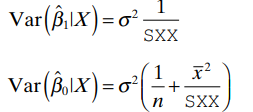
• Variances and Covariances:

The variance of β^₁ is

where σ² is the variance of the errors and Sₓₓ is the sum of squared deviations of x from its mean.

The variance of β^₀​ is

which incorporates both the variability due to the errors and the contribution from the slope estimate.

The covariance between β^₀ and β^₁​ is

​showing that these estimates are generally correlated.

• Correlation Between Estimates: The correlation between β^₀ and β^₁depends on the sample size n and the spread of the x values. Specifically, the correlation can be expressed as:

This correlation is close to ±1 if the variation in x (reflected in Sₓₓ) is small relative to xˉ.

• Gauss–Markov Theorem: This theorem asserts that among all linear unbiased estimators of the regression coefficients, OLS estimators have the smallest variance. Hence, OLS estimates are the Best Linear Unbiased Estimators (BLUE) when the assumptions of the model are satisfied.
• Distributional Assumptions:

For large samples, the OLS estimates are approximately normally distributed due to the Central Limit Theorem.

For small samples with normally distributed errors, the OLS estimates β^₀ and β^₁​ are jointly normally distributed, which also makes them maximum likelihood estimators under normality.

Estimated Variance

Estimates of Var(β^₀ |X) and Var (β^₁| X) are obtained by substituting σ^² for σ²

Estimated Variance

The square root of an estimated variance is called a standard error, for which we use the symbol se( ). The use of this notation is illustrated by

Standard Error

References : Applied Linear Regression, Fourth Edition. Sanford Weisberg. © 2014 John Wiley & Sons, Inc. Published 2014 by John Wiley & Sons, Inc